What is Linear Analysis?
As PEST calibrates a model using its traditional methodology based on finite-difference derivatives of model outputs with respect to parameters, it calculates a Jacobian matrix. This is sometimes called a sensitivity matrix. As such, it represents a linearization of the action of the model on its parameters. Let us refer to this matrix as the “calibration Jacobian matrix”.
PEST can easily be set up to calculate a Jacobian matrix under predictive conditions. This matrix represents a linearization of the action of the model under predictive conditions. Let us call this matrix the “predictive Jacobian matrix”.
Together, the calibration Jacobian matrix and the predictive Jacobian matrix can provide some powerful insights into the flow of information from observations to parameters, and then from parameters to predictions.
When living in a highly-parameterized world (as we must do when working with groundwater models), traditional sensitivity analysis loses its meaning. This is because there is no need to separate parameters which cannot be estimated from those which can, especially when the sensitivities of individual parameter are reduced through the use of many parameters. Furthermore, when it comes to uncertainty analysis, inestimable parameters are just as important as estimable parameters. Moreover, linear analysis demonstrates that the concept of “estimable” should be applied to combinations of parameters rather than to individual parameters. Integrity of separation of parameter space into estimable and inestimable parameter combinations requires the use of lots of parameters.
However while traditional sensitivity analysis is of diminished worth in a highly-parameterized world, linear analysis is not! Some of the insights that it provides can be achieved in no other way.
Many of the utility programs supplied with PEST perform some aspect of linear analysis. Some of the outcomes of these analyses are now described.
Parameter and Predictive Uncertainty
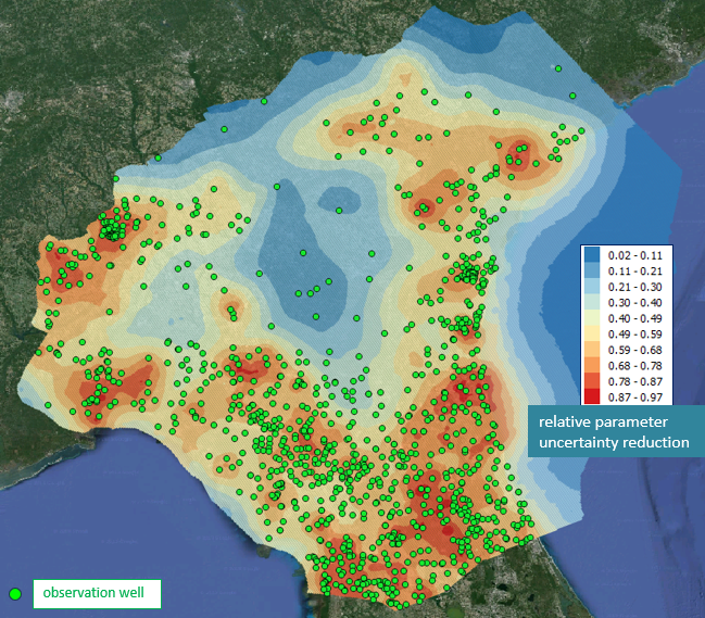
Linear methods can be used to calculate approximate pre-calibration and post-calibration uncertainties of model parameters and model predictions. This type of analysis is sometimes referred to as “first order second moment” or “FOSM” analysis. Armed with this information, maps can be constructed of parameter uncertainty, and of parameter uncertainty reduction. Model stakeholders can then see at a glance where model predictive reliability is high where it is not. They can rapidly relate data density to predictive integrity. The didactic worth of such maps is very high indeed.
Linear analysis supports calculation of the uncertainty of any model prediction. The reduction in its uncertainty accrued through history-matching is also readily calculated.
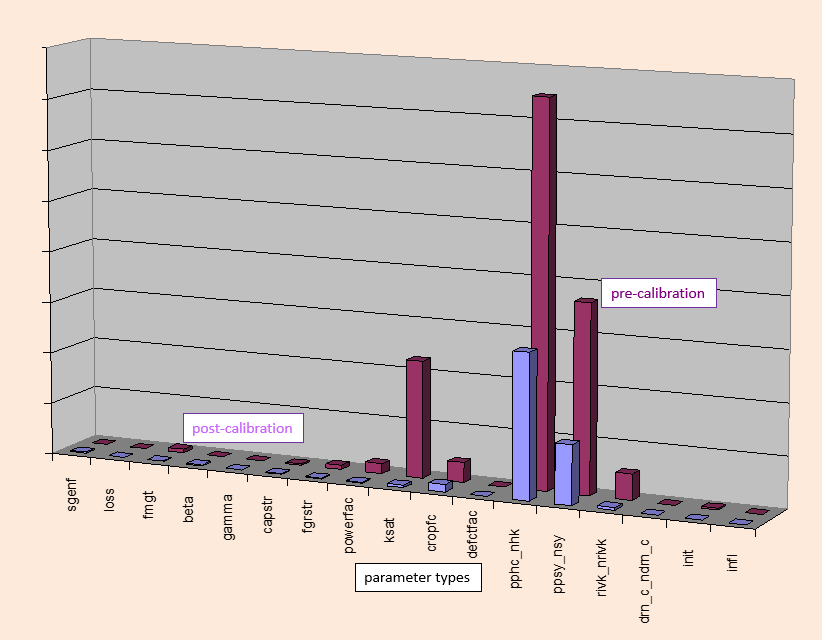
Contributions to Uncertainty
Not only do linear methods allow rapid calculation of the uncertainty of a prediction. They can also calculate contributions to its uncertainty by different parameters, or groups of parameters. These contributions can be those that prevail prior to history matching, or after history matching. Parameters whose contributions are assessed in this way can include not just those that you would adjust when calibrating a model. They can also include specifications of boundary conditions, or other aspects of model design. These “parameters” can be surrogates for an expanded model domain, or for processes which are omitted from a model. The effect of model simplification on its predictive integrity can thereby be assessed. This is especially useful where model simplification has been pursued in order to reduce run times and increase stability. The reduced run times may allow the model to undergo history matching and posterior uncertainty analysis. The cost of achieving this – namely some simplification-induced bias – can be assessed through linear analysis. If the simplicity-induced bias of a prediction is small compared with its uncertainty (of which model simplification has enabled quantification), the benefits of simplification outweigh their costs.
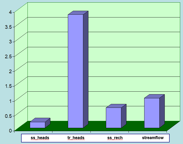
Data Worth
Data has worth in proportion to its ability to reduce the uncertainties of decision-critical model predictions. Linear analysis allows quantification of uncertainty. It also allows easy quantification of uncertainty reduction. In linear analysis, the inclusion or exclusion of data from a history-matching process is simulated by simply adding or removing rows from the calibration Jacobian matrix. Furthermore, the data does not need to exist; linear analysis requires only the sensitivities of corresponding model outcomes to model parameters. The worth of data can thus be quantified before it is acquired.
Other Types of Linear Analysis
Other outcomes of linear analysis supported by utilities available through the PEST suite include the following:
- Flow of information: “super-observations” and “super-parameters”;
- Number of units of information in a calibration dataset;
- Separation of parameter space into orthogonal calibration solution and null spaces;
- Reasons for failure to fit certain components of a calibration dataset;
- Parameter identifiability;
- Composite parameter sensitivities.